
How an Active Fixed Income Strategy Using Yield Curve Positioning May Add Incremental Return.
The Mechanics of “Rolling Down” the Yield Curve
The concept of a bond “rolling down” the yield curve can be a fundamental component of a fixed-income strategy, often referred to as “riding the curve.” This phenomenon describes the potential capital gain a bond generates purely as a result of its remaining time to maturity decreasing, assuming the market’s expectation of future interest rates (the yield curve’s shape) remains constant.
In a normal yield curve environment – where longer maturities offer higher yields than shorter maturities – a bond purchased with a T-year maturity and held for one period will effectively become a (T-1)-year bond. If the yield curve shape does not change, the bond’s new yield-to-maturity (“YTM”) will be lower, corresponding to the shorter maturity. Since bond prices generally move inversely to yields, this decrease in YTM results in capital appreciation for the investor. This price gain, in addition to the coupon payment, constitutes the total return over the holding period.
The roll-down strategy seeks to capitalize on investors initially locking in higher yield of the longer-term bond while only being exposed to the interest rate risk of the shorter holding period.
Impact of Yield Curve Steepness on Roll-Down Performance
The magnitude of the roll-down return is entirely dependent on the steepness of the yield curve at the point the bond is held.
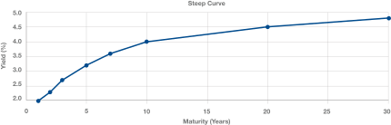
- • Steep Curve (Maximum Roll-Down): A steeply upward-sloping yield curve has historically offered the most significant roll-down opportunity. This typically occurs at the beginning of an economic recovery when the Federal Reserve has kept short-term rates low to stimulate growth, while the market anticipates strong future growth and higher inflation, demanding a much greater term premium for locking up capital long-term.
- o Performance: A steeper curve means the difference in yields is large. As the bond rolls down, its yield drops sharply, resulting in substantial positive capital gains that may boost the total return beyond the coupon yield. Historically, investors have found the “sweet spot” for maximizing this gain is often found in the belly of the curve (e.g., 3-to-7-year maturities), where the curve’s slope is often the steepest.
- o Strategy: Portfolio managers who overweight intermediate (“belly of the curve”) maturities may be designing their portfolios to repeatedly capture roll-down. The emphasis is usually on total return rather than just income.
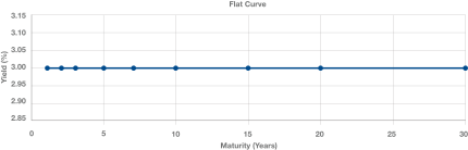
- • Flat Curve (Minimal Roll-Down): A flat curve is one where the yields across all maturities are nearly identical. This has historically signaled market uncertainty or an economy transitioning between phases (e.g., an expansion nearing its end).
- o Performance: The roll-down return is negligible because the difference in yields is near zero. A bond held in this environment primarily derives its return from coupon income, making the roll-down strategy ineffective.
- o Strategy: Portfolio managers will generally take a duration neutral stance and focus on security selection, especially within credit sectors. A barbell strategy may be considered rather than intermediate maturities.
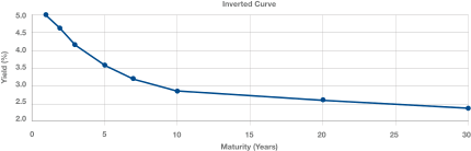
- • Inverted Curve (Negative Roll-Down or “Roll-Up”): An inverted yield curve occurs when short-term yields are higher than long-term yields. Historically associated with late economic cycles or recession expectations.
- o Performance: A bond rolling down the curve moves from a lower long-term yield to a higher short-term yield. This rise in yield results in a capital loss (a “roll-up” loss), as the price of the bond declines, entirely negating the intended benefit of the strategy.
- o Strategy: Portfolio managers may favor shorter duration assets to capture higher front-end yields and reduce reliance on roll-down as a return driver. This will emphasize liquidity and reinvestment flexibility.
Drivers of the Yield Curve Shape: Macro Data and Fed Policy
The shape of the yield curve is governed by the interplay between central bank actions (affecting the short end) and market expectations (affecting the long end).
Federal Reserve Policy (The Short End)
The front end of the curve (maturities of 2 years and less) is primarily influenced by the Federal Reserve’s target for the Federal Funds Rate (“FFR”), the primary monetary policy tool.
- • Rate Hikes: When the Fed raises the FFR to fight inflation (tightening cycle), short-term yields usually follow suit. This action has historically caused the short end of the curve to rise faster than the long end, leading to a flattening or inversion.
- • Rate Cuts: When the Fed cuts the FFR to stimulate a slowing economy (easing cycle), short-term yields generally fall, which has historically led to a steepening of the curve.
Macroeconomic Data (The Long End)
Long-term yields (maturities of 10 years and longer) are driven by the market’s collective forecast for:
- • Inflation Expectations: Usually the single greatest driver of long-term rates. Higher expected inflation erodes the purchasing power of future fixed coupon payments, compelling investors to demand a higher yield (inflation premium) as compensation.
- • Economic Growth: Expectations of robust Gross Domestic Product (“GDP”) growth lead to expectations of greater loan demand by businesses and consumers, and higher future short-term rates, pushing long-term rates higher.
- • Term Premium: An additional risk premium demanded by investors to compensate for the uncertainty of economic conditions over a longer time horizon. A lower term premium flattens the curve, while a higher premium steepens it.

The Inverted Yield Curve and Normalization
Inversion and Significance
A yield curve inversion is a rare and has historically been notable signal of a potential economic recession. Inversion occurs when aggressive Fed tightening causes short-term yields to rise above long-term yields. This typically happens because:
- • Restrictive Policy: Current short-term rates reflect a policy that the market views as overly restrictive, necessary to break inflation.
- • Recession Expectations: The market expects this restrictive policy to trigger a recession, forcing the Fed to cut rates significantly in the future.
- • Flight to Safety: Investors who anticipate a recession or volatility buy long-term bonds (a flight to safety), driving up their prices and pushing their yields down, completing the inversion.
Normalization Over Time
The inverted yield curve will eventually normalize (un-invert) by returning to a normal upward slope. This normalization process typically follows one of two paths, often associated with a final, pre-recession phase:
- • Bull Steepener (The Recession Signal): This is the most common path. The Fed begins to aggressively cut the FFR in response to clear signs of economic weakness. The short end of the curve collapses, falling below the long end, thus restoring the normal slope. Historically, a recession often begins after this un-inversion.
- • Bear Steepener (Rare/Reversal of Trend): This occurs if long-term yields begin to rise significantly (e.g., due to renewed fears of inflation or an unexpected acceleration in growth) while the short end remains high or continues to rise slowly. This normalization suggests the market’s prior expectation of a major slowdown was incorrect.
In many historical market cycles, yield curve normalization has occurred as market expectations for Federal Reserve rate cuts were realized, resulting in a more pronounced decline in short-term yields than long-term yields.

The Current Yield Curve Environment
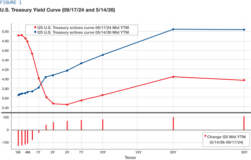
The Federal Reserve began its most recent easing cycle in the second half of 2024, resulting in the FFR declining from 5.50% to a current level of 3.75% as of May 2026. As a result, shorter maturity U.S. Treasury yields dropped 25-100 basis points, while longer dated maturities actually saw yields rise 35 to over 100 basis points. (Source: Bloomberg, U.S. Department of the Treasury.) As a result, the current yield curve environment may present opportunities for active portfolio managers to seek incremental total return through yield curve positioning, depending on market conditions and portfolio objectives. A focus on the belly of the curve could be prudent, as the current curve steepening is more “supply and inflation driven” than “growth optimism driven,” which makes it less supportive for long-duration bonds.
Important Disclosures
This material is provided for informational and educational purposes only and should not be construed as investment advice or a recommendation to buy or sell any security. The discussion reflects market conditions as of the date indicated and is subject to change without notice. Yield curve positioning is an investment technique and does not guarantee positive investment results. Historical market relationships may not persist, and future market conditions may differ materially from those discussed herein.
Independent rating services (such as Standard & Poor’s, Moody’s and Fitch) assign ratings, which generally range from AAA (highest) to D (lowest), to indicate the credit worthiness of the underlying bonds in the portfolio. Where the independent rating services differ in the rating they assign to an issue or do not provide a rating for an issue, the highest available rating is used in calculating allocations by rating. Non-rated bonds are holdings that have not been rated by a nationally recognized statistical rating organization.
The Bloomberg US Corporate High Yield Total Return Index Value Unhedged is an unmanaged index considered representative of the universe of fixed-rate, non-investment grade debt. The Bloomberg U.S. Aggregate Bond Index is an unmanaged index considered representative of the universe of fixed-rate, investment grade taxable debt. Performance of an index does not reflect management fees and expenses which are reflected in Fund performance. An investment cannot be made directly in an index.
BLOOMBERG® is a trademark and service mark of Bloomberg Finance L.P. and its affiliates (collectively “Bloomberg”). Bloomberg or Bloomberg’s licensors own all proprietary rights in the Bloomberg Indices. Bloomberg does not approve or endorse this material or guarantee the accuracy of completeness of any information herein, nor does Bloomberg make any warranty, express or implied, as to the results to be obtained therefrom, and, to the maximum extent allowed by law, Bloomberg shall not have any liability or responsibility for injury or damages arising in connection therewith.
Investing involves risk, including loss of principal. There is no guarantee that any investment strategy will achieve its objectives, generate profits or avoid losses.
Past performance is not indicative of future results. As with any investment vehicle, there is always a potential for profit as well as the possibility of loss. Actual results may differ from composite returns, depending on account size, investment guidelines and/or restrictions, inception date and other factors. Nothing contained in this presentation should be construed as a recommendation to buy or sell a security or economic sector. Please see firm and performance disclosures.
Definitions
Effective Duration measures change in the value of a security in response to a change in interest rates. Weighted Average Maturity refers to the average time it takes for all the bonds within a portfolio to mature, where each bond’s maturity is weighted by its proportion of the total portfolio value. 12-Month Default Rate represents the percentage of bonds outstanding and/or held that have defaulted over the previous 12-month period. Standard Deviation measures that an investment will fluctuate from its expected return. The smaller an investment’s standard deviation, the less volatile it is considered to be. Conversely, the larger the standard deviation, the more volatile the investment. Downside Capture measures manager’s performance in down markets. A down-market is defined as those periods (months or quarters) in which market return is less than 0. Beta is a measure of systematic risk with respect to a benchmark. Beta measures the sensitivity of the fund’s excess return (total return minus the risk-free return) with respect to the benchmark’s excess return that results from their systematic co-movement. The beta of the market is 1.00 by definition.
Material prepared by:
David Schiffman | Portfolio Manager and Director of Fixed Income Investments | Cantor Fitzgerald Asset Management*
*Cantor Fitzgerald Asset Management is the brand name for the asset management business of Cantor Fitzgerald, LP.